Ray Samplers#
Overview#
Once we have a set of cameras, we want to cast camera rays associated with each pixel.
Along these ray we will sample the field and aggregate the samples to predict the pixels value (ie. color). The parameterization of the samples are described here however we must decide where to place these samples along a ray. For this task we will use a Sampler.
In the ideal world we would compute many dense samples along a ray. Unfortunately, each additional sample adds a computation cost to the system as it needs to be processed by the field which is often a neural network.
As a result it is common for NeRF methods to use on the order of 100 samples. Therefore, we want to optimize where those samples are placed in the scene.
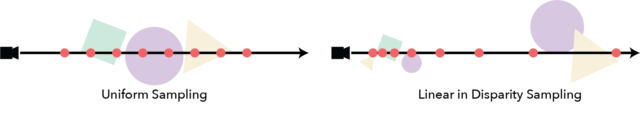
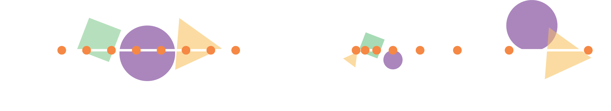
For example, if the scene can be bounded by a box and the objects are all similar scales, uniform sampling along the ray may be a good option. On the other hand if the scene is unbounded (potential extending as far as the eye can see) uniform sampling does not make sense as the samples would be very sparse for close objects. In this case a different sampling like Uniform in Disparity may perform better.
Stratified Sampling#
Most samplers has the option to stratify the samplers. When stratified, each sample is randomly perturbed.
The magnitude of the pertubation is such that the sample ordering remains consistent and the overall distribution statistics are not changed. Using stratified samples during training generally improves the reconstructions as it help prevent overfitting.
During inference stratified sampling should be disabled (nerfstudio samplers will do this) as it can cause noisy artifacts when the camera moves.


Hierarchical Sampling#
It is important to sample the scene where it has content otherwise the reconstruction quality will be reduced.
One trick that is often employed in NeRF methods is to do multiple round of sampling. The first round can use a predefined sampler (ie. Uniform) to generate an image. Once the space is sampled, we have an idea which samples contributed to the final color.
We can use this information to sample more around those regions using a PDFSampler. The PDF sampler is described more below.
Spaced Samplers#
These are the most basic samplers that spaces samples based on a predefined function. These samplers have all have a starting and ending distance (also known as a near/far plane). The plots below are histograms of points sampled from some predefined samplers.
# COLLAPSED
import plotly.graph_objects as go
import torch
from plotly.subplots import make_subplots

from nerfstudio.cameras.rays import RayBundle
from nerfstudio.model_components import ray_sampler

num_samples = 1000
near = 2
far = 5
train_stratified = False

samplers = [
    ray_sampler.UniformSampler,
    ray_sampler.LinearDisparitySampler,
    ray_sampler.SqrtSampler,
    ray_sampler.LogSampler,
]

fig = make_subplots(
    rows=2,
    cols=2,
    subplot_titles=("Uniform", "Linear in Disparity", "Square Root", "Log Sampler"),
    shared_xaxes=True,
    shared_yaxes=True,
    vertical_spacing=0.1,
)

for i, Sampler in enumerate(samplers):
    sampler = Sampler(num_samples=num_samples, train_stratified=train_stratified)

    ray_bundle = RayBundle(
        origins=torch.ones([1, 3]),
        directions=torch.ones([1, 3]),
        pixel_area=torch.ones([1, 1]),
        nears=torch.ones([1, 1]) * near,
        fars=torch.ones([1, 1]) * far,
    )

    samples = sampler.generate_ray_samples(ray_bundle)

    trace = go.Histogram(x=samples.frustums.starts[0, :, 0], nbinsx=50)
    fig.append_trace(trace, i // 2 + 1, i % 2 + 1)

fig.update_yaxes(title_text="# Samples", row=1, col=1)
fig.update_yaxes(title_text="# Samples", row=2, col=1)
fig.update_xaxes(title_text="Distance", row=2, col=1)
fig.update_xaxes(title_text="Distance", row=2, col=2)

# Overlay both histograms
fig.update_layout(height=700, hovermode=False, showlegend=False, margin=dict(l=20, r=20, t=50, b=20))
fig.update_yaxes(range=[0, 80])
fig.update_traces(opacity=0.7)
fig.show()
PDF Sampler#
The Probability Distribution Function (PDF) Sampler generates samples that match a given distribution.
In the example below we first create a UniformSampler to generate a set of initial samples. We then assign weights to each of these samples to define the PDF (here it is an arbitrary function, but usually you would use the predicted weights from the field). The left plot the target PDF, on the right we plot a histogram of samples generated from the PDFSampler.
# COLLAPSED
import plotly.graph_objects as go
import torch
from plotly.subplots import make_subplots

from nerfstudio.cameras.rays import RayBundle
from nerfstudio.model_components import ray_sampler

num_coarse_samples = 20
num_samples = 1000
near = 2
far = 5
train_stratified = False

fig = make_subplots(
    rows=1,
    cols=2,
    subplot_titles=("PDF", "Samples"),
)

uniform_sampler = ray_sampler.UniformSampler(num_samples=num_coarse_samples, train_stratified=train_stratified)
pdf_sampler = ray_sampler.PDFSampler(num_samples=num_samples, train_stratified=train_stratified, include_original=False)

ray_bundle = RayBundle(
    origins=torch.ones([1, 3]),
    directions=torch.ones([1, 3]),
    pixel_area=torch.ones([1, 1]),
    nears=torch.ones([1, 1]) * near,
    fars=torch.ones([1, 1]) * far,
)

coarse_ray_samples = uniform_sampler(ray_bundle)

# Generate arbitrary PDF
weights = torch.ones(num_coarse_samples)
weights += torch.sin(torch.linspace(0, 3 * torch.pi, num_coarse_samples))
weights += torch.sin(torch.linspace(0, 0.5 * torch.pi, num_coarse_samples))
weights -= torch.min(weights)
weights /= torch.sum(weights)

samples = pdf_sampler.generate_ray_samples(ray_bundle, coarse_ray_samples, weights[None, :, None], num_samples)

# Plotting stuff
x = torch.ones((num_coarse_samples * 2))
x[::2] = coarse_ray_samples.frustums.starts[0, :, 0]
x[1::2] = coarse_ray_samples.frustums.ends[0, :, 0]

y = torch.ones((num_coarse_samples * 2))
y[::2] = weights
y[1::2] = weights

pdf_trace = go.Scatter(x=x, y=y)
fig.append_trace(pdf_trace, 1, 1)

samples_trace = go.Histogram(x=samples.frustums.starts[0, :, 0], nbinsx=100)
fig.append_trace(samples_trace, 1, 2)

fig.update_yaxes(title_text="# Samples", row=1, col=2)
fig.update_xaxes(title_text="Distance", row=1, col=1)
fig.update_xaxes(title_text="Distance", row=1, col=2)

# Overlay both histograms
fig.update_layout(height=400, hovermode=False, showlegend=False, margin=dict(l=20, r=20, t=50, b=20))
fig.update_traces(opacity=0.7)
fig.show()